Akvorado vs GoFlow2 + Loki: Same NetFlow, Two Stacks

There are two ways to get NetFlow into a dashboard. One is a purpose-built flow tool like Akvorado. The other is a small collector such as GoFlow2 that writes JSON, plus a log stack like Loki and Grafana that you may already run. I had both receiving the same NetFlow v9 export from two Cisco IOS XE 17.18.2 routers, so I compared them on the same 15 minutes of traffic. I looked at whether the numbers agree, what each one costs to run, and where the lighter stack falls short. All of it was built in my home lab.

The setups are in earlier posts: Akvorado on Cisco IOS XE and NetFlow and IPFIX in Grafana. The traffic is the bandwidth-hog scenario from Troubleshooting with NetFlow: who is eating the WAN?

The versions

• Akvorado v2026.10.1 (AGPL-3.0), with Kafka 4.3.1 and ClickHouse 26.3.
• GoFlow2 v2.2.5-39-gc640271 (BSD-3-Clause), from the netsampler/goflow2:latest image.
• Grafana Alloy v1.21.3 (Apache-2.0) tails the GoFlow2 file and ships it.
• Loki 3.7.9 and Grafana 13.0.2 (both AGPL-3.0).

Everything is free to run. None of these has a paid tier that you need for this.

One export, two collectors

A single flow monitor on each router feeds both collectors. Flexible NetFlow lets one monitor reference more than one exporter, so the routers build each flow once and send it twice:

flow monitor AKV-MON
 exporter AKV-EXP
 exporter GF2-EXP
 record AKV-REC
!
interface Ethernet0/1
 ip flow monitor AKV-MON input
interface Ethernet0/2
 ip flow monitor AKV-MON input

AKV-EXP points at the Akvorado inlet and GF2-EXP at GoFlow2, both on UDP 2055. Because both collectors get identical records, any difference in the results comes from the collectors, not the routers.

The lighter stack

GoFlow2 has no config file here. It's run with three flags:

goflow2 -listen=netflow://:2055 -format=json -transport=file -transport.file=/flows/flows.log

Each flow becomes one JSON line with fields like sampler_address, src_addr, dst_addr, proto, bytes, in_if and out_if. Alloy tails that file and promotes only the exporter address to a Loki label. Everything else stays in the log line, which keeps label cardinality low:

local.file_match "flows" {
  path_targets = [{"__path__" = "/flows/flows.log", job = "netflow"}]
}

loki.source.file "flows" {
  targets    = local.file_match.flows.targets
  forward_to = [loki.process.flows.receiver]
}

loki.process "flows" {
  stage.json {
    expressions = { exporter = "sampler_address" }
  }
  stage.labels {
    values = { exporter = "" }
  }
  forward_to = [loki.write.local.receiver]
}

Grafana then does the math at query time with LogQL. Here's the "bits per second leaving the WAN, by source" panel:

sum by (src_addr) (
  sum_over_time({job="netflow", exporter="10.66.20.11"}
    | json | out_if="2" | unwrap bytes [1m])
) * 8 / 60

Note the out_if="2". GoFlow2 only knows interface indexes, so I had to look up that Ethernet0/1 is ifIndex 2 on wan-rtr1 with show snmp mib ifmib ifindex. Akvorado gets the name, description and speed over SNMP and lets you filter on OutIfName = 'Et0/1', or on a boundary such as "external".

Same 15 minutes, side by side

Both views cover 21:55 to 22:10 Pacific, wan-rtr1 only, traffic leaving Et0/1.

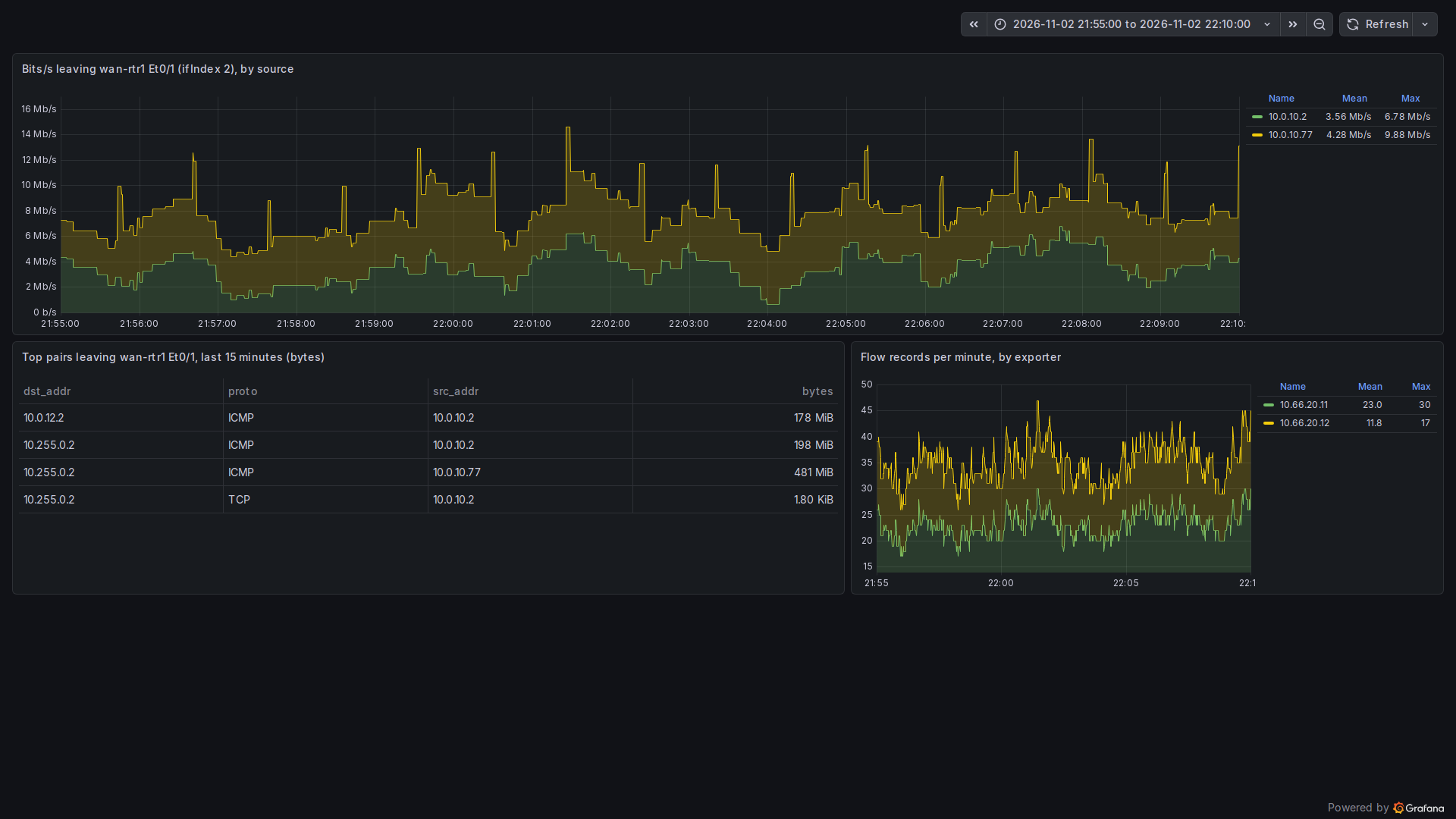
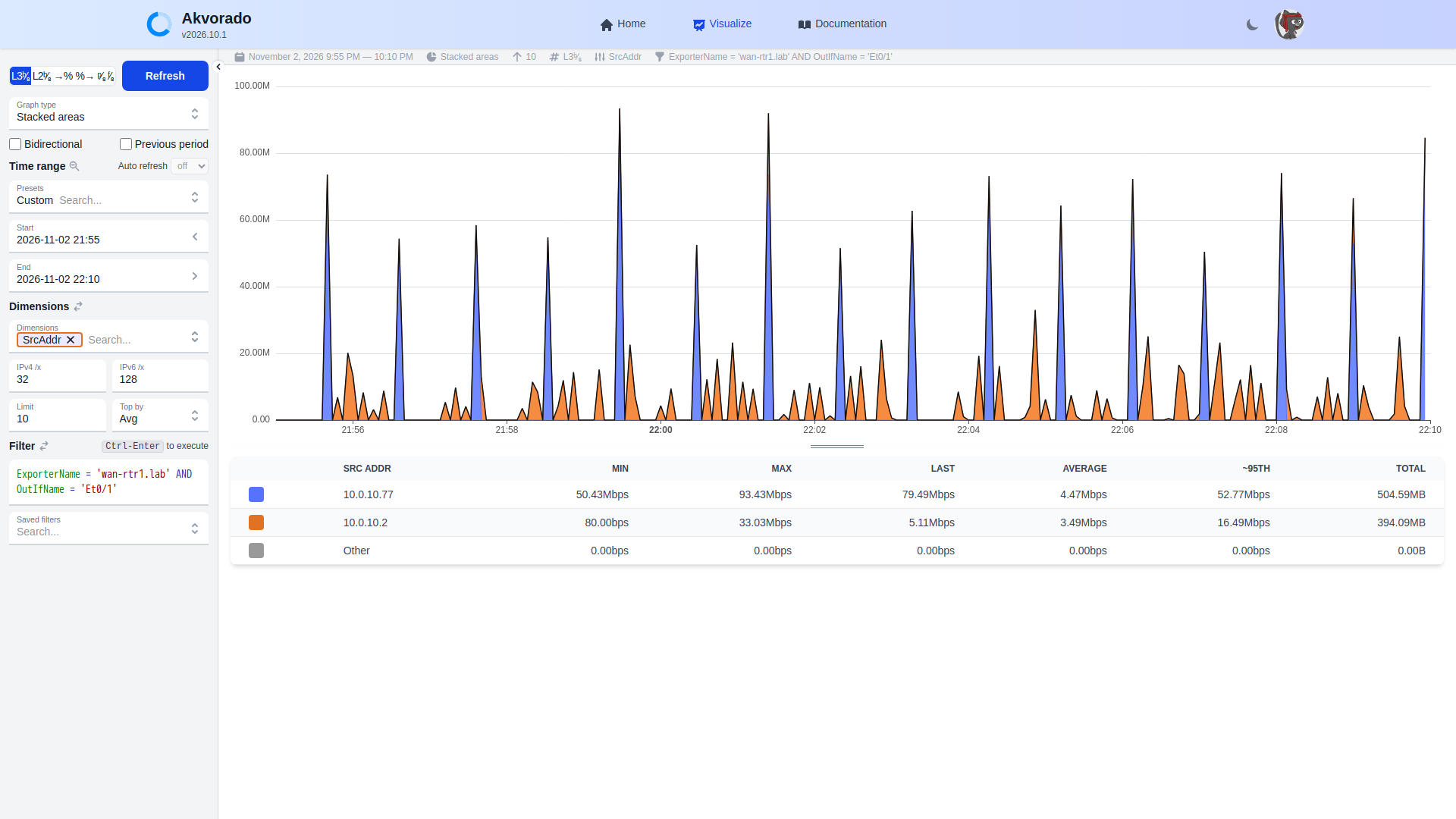
The shapes look nothing alike, and that's expected. Akvorado puts each flow's bytes at the moment the flow was received, so every 40-second ping run shows as one tall spike. The LogQL query sums over a sliding one-minute window, which spreads each flow out and gives a smoother line. The means differ slightly because the two tools bucket time differently. Neither graph is wrong, but neither is the real per-second rate. With a 1800-second active timeout, which is all this IOS XE image allows, the peaks are approximate in any tool.

The totals tell you whether the collectors agree. Here's ClickHouse, under Akvorado:

SELECT replaceOne(toString(SrcAddr), '::ffff:', '') AS src,
       replaceOne(toString(DstAddr), '::ffff:', '') AS dst,
       count() AS flows, sum(Bytes) AS bytes
FROM flows
WHERE TimeReceived >= toDateTime('2026-11-03 05:55:00', 'UTC')
  AND TimeReceived <  toDateTime('2026-11-03 06:10:00', 'UTC')
  AND ExporterName = 'wan-rtr1.lab' AND OutIfName = 'Et0/1'
GROUP BY src, dst ORDER BY bytes DESC LIMIT 5

src          dst          flows  bytes
10.0.10.77   10.255.0.2      16  504586500
10.0.10.2    10.255.0.2      75  207487444
10.0.10.2    10.0.12.2       44  186598700

And here's Loki, with the same window ending at 22:10 Pacific:

topk(5, sum by (src_addr, dst_addr) (
  sum_over_time({job="netflow", exporter="10.66.20.11"}
    | json | out_if="2" | unwrap bytes [15m])))

10.0.10.77   10.255.0.2   504586500
10.0.10.2    10.255.0.2   207487444
10.0.10.2    10.0.12.2    186598700

They match to the byte. Record counts match too: 346 flow records from wan-rtr1 and 177 from wan-rtr2 in both stores. On accuracy there's nothing to choose between them. The two collectors decode the same NetFlow v9 records into the same numbers. I trimmed the ClickHouse table borders, and the time filter is in UTC because that's how TimeReceived is stored.

What each one costs to run

Memory from docker stats, taken once while both were receiving the same export (Grafana isn't counted for either side):

Akvorado stack                       GoFlow2 + Loki stack
clickhouse      707.8 MiB            pl-loki       96.3 MiB
kafka          1004.0 MiB            pl-alloy      41.1 MiB
kafka-ui        644.8 MiB            pl-goflow2     8.7 MiB
inlet            32.3 MiB
outlet           23.0 MiB
traefik          29.2 MiB
console          16.3 MiB
orchestrator     13.3 MiB
redis             4.6 MiB

That's about 2.4 GiB against about 146 MiB. You can drop kafka-ui, which is only a web UI for Kafka, and bring Akvorado down to about 1.8 GiB. Kafka and ClickHouse are most of the cost, and they're also what lets Akvorado handle a busy network. At two routers and a few hundred flows a minute, it's mostly idle capacity.

Storage goes the other way. ClickHouse held 1,334 raw flows in about 37 KiB on disk, plus three small rollup tables. GoFlow2's JSON file was 1.4 MB for about 1,448 lines, and the Loki volume was 1.7 MB. That Loki number includes syslog from the same routers, so it isn't a clean comparison. Still, columnar storage is far more compact than JSON lines, and the gap grows with volume.

Where the lighter stack runs out

• No interface names or descriptions. You filter on ifIndex numbers and keep a mapping somewhere. ifIndex can change after a reload unless you configure snmp ifmib ifindex persist.
• No classification. Akvorado tags exporters by site and role, interfaces by boundary, and addresses by network name. In LogQL you rebuild that by hand with label filters and regular expressions in every query.
• Query cost grows with time range. Every LogQL query parses JSON at read time. Fifteen minutes of a small lab is instant. A month of a real WAN means a lot of log lines to parse. Akvorado answers long ranges from pre-built 1-minute, 5-minute and 1-hour rollup tables.
• Double counting is easier to miss. Both tools see the same packets from both routers. Akvorado's exporter and boundary dimensions make that obvious. In Loki you need to remember the exporter label every time.

Where it wins

• It's tiny: three small processes and about 146 MiB of RAM.
• If you already run Loki and Grafana, you add one container and a few lines of Alloy config.
• Flows sit in the same Grafana as your SNMP graphs and syslog, so you can put "interface is busy" and "who is using it" on one dashboard.
• The raw JSON is easy to grep or feed into something else.

Which one I'd pick

For a single site or a handful of routers where someone occasionally asks "who used the link", GoFlow2 into Loki is enough. It's the one I'd set up first. Once flows become a daily tool, with several sites, people other than you asking questions, or anything past a few days of history, Akvorado's enrichment and storage are worth the extra RAM.

If you're not sure which NetFlow version to export, NetFlow versions compared covers v5, v9 and IPFIX. The router-side setup is in Flexible NetFlow on Cisco IOS XE.

Next in this series: using the same flow data for security, to spot scans, odd ports and traffic that shouldn't be there.

Now live: Security from NetFlow: spotting scans and sweeps.